How to Read Spss T Test Output
The t-test process performs t-tests for one sample, 2 samples and paired observations. The single-sample t-test compares the mean of the sample to a given number (which you supply). The independent samples t-test compares the difference in the means from the 2 groups to a given value (commonly 0). In other words, information technology tests whether the difference in the means is 0. The dependent-sample or paired t-test compares the deviation in the means from the two variables measured on the same set of subjects to a given number (usually 0), while taking into account the fact that the scores are not independent. In our examples, we volition use the hsb2 data set.
Unmarried sample t-test
The single sample t-test tests the null hypothesis that the population mean is equal to the number specified by the user. SPSS calculates the t-statistic and its p-value nether the assumption that the sample comes from an approximately normal distribution. If the p-value associated with the t-exam is small (0.05 is often used as the threshold), there is testify that the mean is different from the hypothesized value. If the p-value associated with the t-test is not small (p > 0.05), so the null hypothesis is non rejected and y'all can conclude that the mean is not unlike from the hypothesized value.
In this example, the t-statistic is 4.140 with 199 degrees of freedom. The corresponding two-tailed p-value is .000, which is less than 0.05. Nosotros conclude that the mean of variable write is different from 50.
get file "C:\data\hsb2.sav".
t-test /testval=50 variables=write.
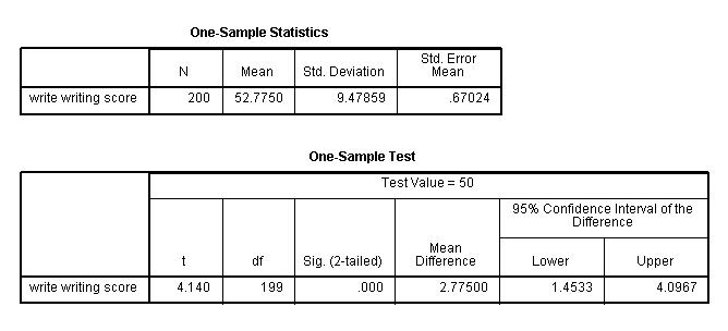
One-Sample Statistics
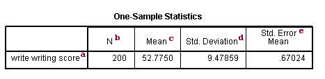
a. – This is the list of variables. Each variable that was listed on the variables= statement in the above lawmaking will have its own line in this part of the output.
b. Northward – This is the number of valid (i.e., not-missing) observations used in calculating the t-test.
c. Mean – This is the mean of the variable.
d. Std. Deviation – This is the standard difference of the variable.
e. Std. Error Mean – This is the estimated standard difference of the sample mean. If we drew repeated samples of size 200, we would expect the standard departure of the sample ways to be close to the standard error. The standard deviation of the distribution of sample mean is estimated as the standard deviation of the sample divided by the foursquare root of sample size: 9.47859/(sqrt(200)) = .67024.
Test statistics
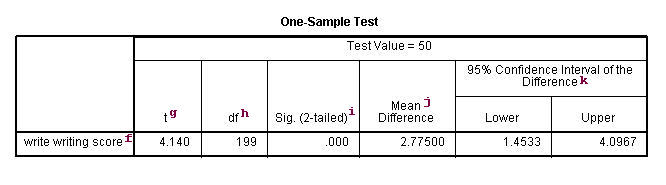
f. – This identifies the variables. Each variable that was listed on the variables= statement will have its own line in this part of the output. If a variables= argument is not specified, t-test will behave a t-examination on all numerical variables in the dataset.
k. t – This is the Educatee t-statistic. Information technology is the ratio of the departure betwixt the sample mean and the given number to the standard mistake of the hateful: (52.775 – 50) / .6702372 = four.1403. Since the standard fault of the hateful measures the variability of the sample hateful, the smaller the standard mistake of the hateful, the more likely that our sample mean is close to the true population mean. This is illustrated by the following three figures.
In all three cases, the difference between the population means is the same. But with large variability of sample ways, second graph, two populations overlap a great deal. Therefore, the difference may well come by take a chance. On the other mitt, with pocket-sized variability, the deviation is more than clear as in the tertiary graph. The smaller the standard error of the hateful, the larger the magnitude of the t-value and therefore, the smaller the p-value.
h.df – The degrees of freedom for the unmarried sample t-test is but the number of valid observations minus one. We loose one caste of freedom because nosotros have estimated the hateful from the sample. We have used some of the information from the data to estimate the mean, therefore it is not available to use for the test and the degrees of freedom accounts for this.
i. Sig (2-tailed)– This is the two-tailed p-value evaluating the null against an alternative that the mean is non equal to 50. It is equal to the probability of observing a greater absolute value of t nether the cypher hypothesis. If the p-value is less than the pre-specified blastoff level (ordinarily .05 or .01) we volition conclude that mean is statistically significantly dissimilar from nada. For case, the p-value is smaller than 0.05. And then we conclude that the mean forwrite is different from 50.
j. Mean Difference – This is the difference betwixt the sample mean and the test value.
k. 95% Confidence Interval of the Difference – These are the lower and upper bound of the confidence interval for the mean. A confidence interval for the mean specifies a range of values within which the unknown population parameter, in this case the mean, may lie. It is given by
![]()
where s is the sample deviation of the observations and N is the number of valid observations. The t-value in the formula can be computed or constitute in any statistics book with the degrees of liberty existence Northward-ane and the p-value being 1-blastoff/ii, where alpha is the confidence level and by default is .95.
Paired t-test
A paired (or "dependent") t-examination is used when the observations are not independent of ane some other. In the example below, the same students took both the writing and the reading exam. Hence, y'all would expect there to exist a relationship between the scores provided by each student. The paired t-test accounts for this. For each student, we are essentially looking at the differences in the values of the two variables and testing if the hateful of these differences is equal to nada.
In this case, the t-statistic is 0.8673 with 199 degrees of freedom. The respective two-tailed p-value is 0.3868, which is greater than 0.05. We conclude that the mean difference of write and read is not different from 0.
t-exam pairs=write with read (paired).
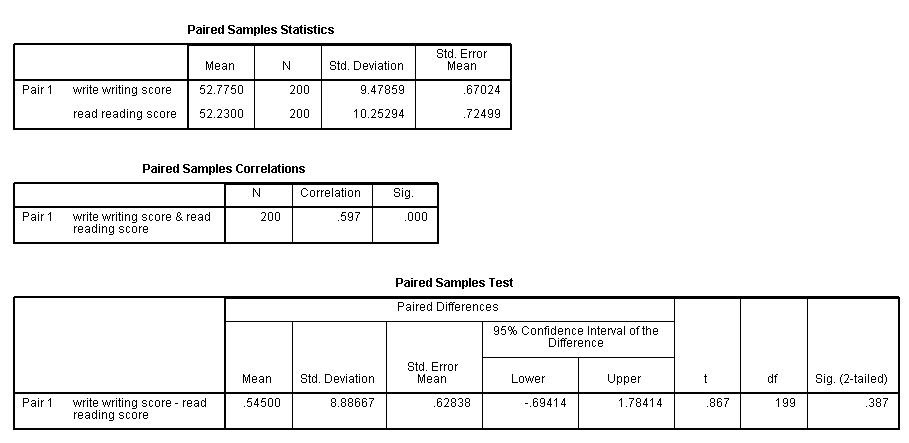
Summary statistics
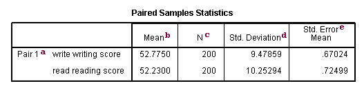
a. – This is the list of variables.
b. Mean – These are the corresponding means of the variables.
c. Northward – This is the number of valid (i.eastward., not-missing) observations used in computing the t-examination.
d. Std. Difference – This is the standard deviations of the variables.
east. Std Error Mean – Standard Error Mean is the estimated standard deviation of the sample hateful. This value is estimated equally the standard deviation of one sample divided by the square root of sample size: ix.47859/sqrt(200) = .67024, 10.25294/sqrt(200) = .72499. This provides a measure of the variability of the sample hateful.
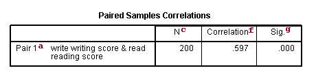
f. Correlation – This is the correlation coefficient of the pair of variables indicated. This is a mensurate of the strength and direction of the linear relationship between the two variables. The correlation coefficient can range from -1 to +1, with -1 indicating a perfect negative correlation, +1 indicating a perfect positive correlation, and 0 indicating no correlation at all. (A variable correlated with itself will always have a correlation coefficient of one.) You can think of the correlation coefficient as telling you the extent to which you can estimate the value of ane variable given a value of the other variable. The .597 is the numerical clarification of how tightly around the imaginary line the points prevarication. If the correlation was higher, the points would tend to be closer to the line; if it was smaller, they would tend to be further abroad from the line.
g. Sig – This is the p-value associated with the correlation. Hither, correlation is significant at the .05 level.
Test statistics
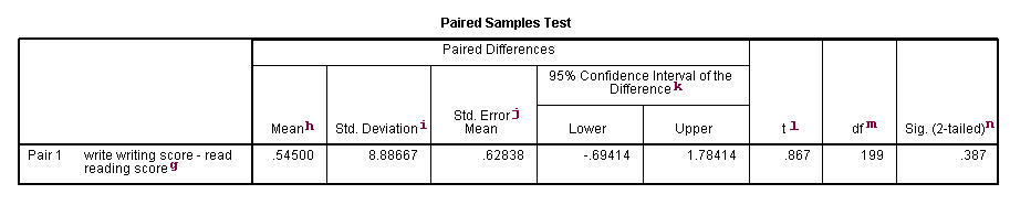
g. writing score-reading score – This is the value measured within each discipline: the deviation between the writing and reading scores. The paired t-test forms a single random sample of the paired departure. The mean of these values among all subjects is compared to 0 in a paired t-test.
h. Mean – This is the mean within-subject difference between the two variables.
i. Std. Deviation – This is the standard deviation of the mean paired difference.
j. Std Error Mean – This is the estimated standard deviation of the sample mean. This value is estimated as the standard departure of one sample divided by the square root of sample size: 8.88667/sqrt(200) = .62838. This provides a measure of the variability of the sample hateful.
k. 95% Confidence Interval of the Divergence – These are the lower and upper bound of the confidence interval for the mean difference. A confidence interval for the mean specifies a range of values inside which the unknown population parameter, in this case the hateful, may prevarication. It is given by
![]()
where s is the sample deviation of the observations and N is the number of valid observations. The t-value in the formula can exist computed or institute in any statistics volume with the degrees of freedom being Due north-1 and the p-value being 1-blastoff/2, where alpha is the confidence level and by default is .95.
fifty. t – This is the t-statistic. Information technology is the ratio of the mean of the difference to the standard error of the deviation: (.545/.62838).
one thousand. degrees of freedom – The degrees of freedom for the paired observations is simply the number of observations minus 1. This is because the examination is conducted on the one sample of the paired differences.
due north. Sig. (2-tailed) – This is the two-tailed p-value computed using the t distribution. Information technology is the probability of observing a greater accented value of t under the goose egg hypothesis. If the p-value is less than the pre-specified alpha level (usually .05 or .01, here the onetime) we will conclude that mean departure between writing score and reading score is statistically significantly different from aught. For example, the p-value for the difference between the two variables is greater than 0.05 so nosotros conclude that the mean difference is not statistically significantly different from 0.
Contained group t-test
This t-test is designed to compare means of same variable between two groups. In our example, we compare the mean writing score between the group of female students and the group of male person students. Ideally, these subjects are randomly selected from a larger population of subjects. The test assumes that variances for the two populations are the same. The interpretation for p-value is the aforementioned equally in other type of t-tests.
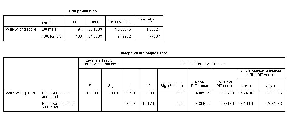
In this example, the t-statistic is -3.7341 with 198 degrees of freedom. The corresponding 2-tailed p-value is 0.0002, which is less than 0.05. We conclude that the difference of means in write between males and females is different from 0.
t-test groups=female(0 1) /variables=write.
Summary statistics
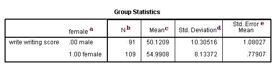
a. female – This column gives categories of the independent variable female. This variable is necessary for doing the independent group t-test and is specified past the t-test groups= statement.
b. Northward – This is the number of valid (i.east., not-missing) observations in each group.
c. Hateful – This is the mean of the dependent variable for each level of the contained variable.
d. Std. Deviation – This is the standard deviation of the dependent variable for each of the levels of the independent variable.
e. Std. Mistake Mean – This is the standard error of the mean, the ratio of the standard deviation to the square root of the respective number of observations.
Exam statistics
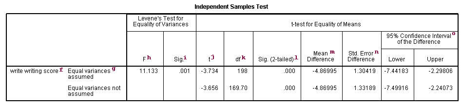
f. – This cavalcade lists the dependent variable(s). In our example, the dependent variable is write (labeled "writing score").
k. – This column specifies the method for computing the standard error of the departure of the means. The method of computing this value is based on the assumption regarding the variances of the ii groups. If we assume that the ii populations have the same variance, and so the first method, called pooled variance reckoner, is used. Otherwise, when the variances are not assumed to exist equal, the Satterthwaite's method is used.
h. F– This column lists Levene'south test statistic. Assume \(yard\) is the number of groups, \(N\) is the total number of observations, and \(N_i\) is the number of observations in each \(i\)-th group for dependent variable \(Y_{ij}\). Then Levene's test statistic is defined equally
\brainstorm{equation} W = \frac{(N-k)}{(k-1)} \frac{\sum_{i=1}^{k} N_i (\bar{Z}_{i.}-\bar{Z}_{..})^two}{\sum_{i=1}^{thou}\sum_{j=1}^{N_i}(Z_{ij}-\bar{Z}_{i.})^two} \terminate{equation}
\begin{equation} Z_{ij} = |Y_{ij}-\bar{Y}_{i.}| \cease{equation}
where \(\bar{Y}_{i.}\) is the mean of the dependent variable and \(\bar{Z}_{i.}\) is the hateful of \(Z_{ij}\) for each \(i\)-thursday group respectively, and \(\bar{Z}_{..}\) is the thou mean of \(Z_{ij}\).
i. Sig. – This is the two-tailed p-value associated with the null that the two groups accept the same variance. In our example, the probability is less than 0.05. So in that location is show that the variances for the two groups, female person students and male students, are different. Therefore, we may want to use the 2d method (Satterthwaite variance figurer) for our t-test.
j. t – These are the t-statistics under the two different assumptions: equal variances and unequal variances. These are the ratios of the hateful of the differences to the standard errors of the divergence nether the two different assumptions: (-iv.86995 / 1.30419) = -3.734, (-4.86995/1.33189) = -3.656.
k. df – The degrees of freedom when we presume equal variances is only the sum of the ii sample sized (109 and 91) minus 2. The degrees of freedom when we assume unequal variances is calculated using the Satterthwaite formula.
l. Sig. (ii-tailed) – The p-value is the two-tailed probability computed using the t distribution. It is the probability of observing a t-value of equal or greater accented value under the zippo hypothesis. For a one-tailed examination, halve this probability. If the p-value is less than our pre-specified alpha level, usually 0.05, nosotros will conclude that the divergence is significantly dissimilar from zero. For case, the p-value for the deviation between females and males is less than 0.05 in both cases, so we conclude that the difference in means is statistically significantly dissimilar from 0.
g. Mean Deviation – This is the difference between the means.
n. Std Error Departure – Standard Fault difference is the estimated standard deviation of the difference between the sample ways. If we drew repeated samples of size 200, we would expect the standard departure of the sample means to exist close to the standard fault. This provides a measure of the variability of the sample mean. The Fundamental Limit Theorem tells us that the sample means are approximately normally distributed when the sample size is thirty or greater. Note that the standard error divergence is calculated differently under the two dissimilar assumptions.
o.95% Conviction Interval of the Divergence – These are the lower and upper bound of the confidence interval for the mean difference. A confidence interval for the mean specifies a range of values inside which the unknown population parameter, in this instance the mean, may lie. Information technology is given by
![]()
where s is the sample deviation of the observations and N is the number of valid observations. The t-value in the formula can exist computed or found in any statistics book with the degrees of freedom being N-i and the p-value beingness 1-width/2, where width is the confidence level and past default is .95.
How to Read Spss T Test Output
Source: https://stats.oarc.ucla.edu/spss/output/t-test/
0 Response to "How to Read Spss T Test Output"
Post a Comment